5.7. RANSAC Paradigm

The RANSAC plgorithm was first introduced by Fischler and Bolles in [FischlerBolles1981].

5.7.1. Video

This is a nice explanation by Behnam Asadi from YouTube.

5.7.2. RANSAC is Not Least Trimmed Squares

Typically in Least Squares (LS) fitting, we use all the data to fit a model.
In Least Trimmed Squares, you compute LS, throw away a percentage of bad data, then recompute, and repeat.
Fischler and Bolles show, this can still fail, as the initial model can be affected by the bad data.
They wanted a more robust method.

5.7.3. The Paradigm

Given a model that requires a minimum of $n$ points to compute a solution, and a set of data points $P$ where $\#(P) \ge n$ :

Select a random subset of $n$ data points from $P$ to form $S1$
Instantiate the model $M1$
Determine the set $S1*$ within error threshold of model $M1$ , and count the members of $S1*$ . This is the consensus set.
If $\#(S1*)$ greater than a threshold $t$ , use $S1*$ to compute a new model $M1*$
If $\#(S1*)$ is less than $t$ , select a new random subset $S2$ and repeat.
If after $k$ iterations, no consensus set with $t$ or more members has been found, solve with the largest consensus set, or terminate with failure.

Parameters:

$e$ : error threshold to determine which points are inliers
$t$ : minimum number of inliers to accept as forming a valid model
$k$ : number of iterations to try

Referring to paper:

$w$ : probability that any given point is within error tolerance of model
$z$ : certainty that at least one of our subsets contains error free data

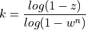
So,

$( 1 - w^n )^k = ( 1 - z)$

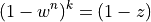
gives:

$k = \frac{log(1-z)}{log(1-w^n)}$

For example, if we think that 20 percent of the data is bad, the probability of picking a good data point is $w = 0.8$ . If we want 99 percent confidence that we will end up with a good model then, $z = 0.99$ . So, in a line fitting problem, $n = 2$ , so the number of iterations $k$ we should attempt should be:

$k = \frac{log(1-0.99)}{log(1-0.8^2)}$

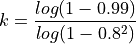
which is $k = 4.5$ , so at least 5 iterations should be made.

Alternatively, the paper derives the expectation of $k$ as:

$E(k) = w^{-n}$

and the standard deviation of $k$ to be:

$SD(k) = (sqrt(1 - w^n)) * (1 / w^n)$

which in the same example gives, a mean of 1.56, a SD of 0.9, so if we wanted mean plus 3 standard deviations, its we’d need 5 iterations again.

With poor data, say $w = 0.5$ , we’d need approx 16 iterations.

From [FischlerBolles1981], you could terminate early the first time you get a consensus set larger than a minimum size, i.e. threshold $t$ , or if you don’t get over $t$ , just pick the largest consensus set you found.

It depends if you want to finish early, or fit the most data, so in practice, implementations may differ.

For another explanation, see Ziv Yaniv’s example, which uses RANSAC to solve for parameters of a hyperplane and hypersphere, and discusses various implementation details.

5.7.4. Widely Applicable

It’s not a specific algorithm
It’s a way of solving model fitting problems
So, problem and implementation specific
e.g. Pivot calibration, pose estimation, line fitting

5.7.5. Notebooks

Have a play with the provided Jupyter Notebooks.

scikit-surgery provides the main algorithms:

# Note that the scikit-surgery libraries provide pivot and RANSAC.
import sksugerycalibration.algorithms.pivot as p   # AOS Pivot algorithm and a RANSAC version.
import sksurgerycore.transforms.matrix as m  # For creating 4x4 matrices.

so the algorithms are here and the matrix utilities are here.

and can be installed with:

pip install scikit-surgerycalibration